Automatic extraction of reproducible semi-quantitative histological metrics for MRI-histology correlations
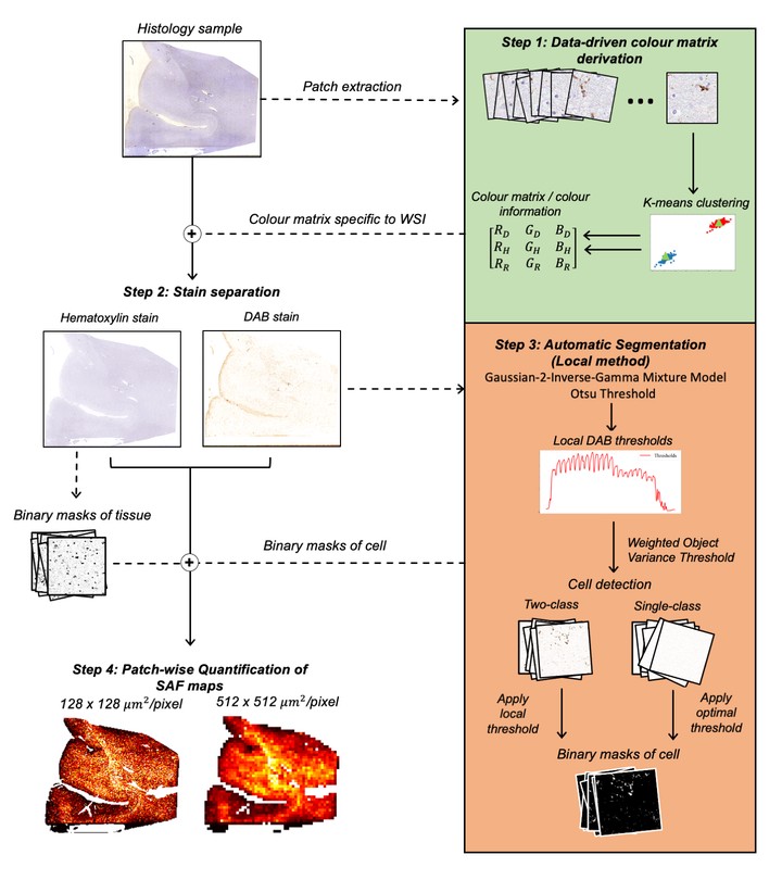 Image credit: Daniel Kor
Introduction:
Comparison of MRI to stained tissue slides from the same sample provides insight into the cellular and molecular correlates of MRI signals, which are notoriously non-specific. Immunohistochemistry (IHC) is a histological staining technique that uses diaminobenzidine (DAB) to stain a target protein brown, and hematoxylin to counterstain background tissue purple. While many studies use IHC to validate MR measures, there is no standardised pipeline for extracting quantitative metrics from IHC slides, with most analyses requiring manual intervention1,2,3.
The stained area fraction (SAF) is a common metric that counts how many pixels in a digitised slide correspond to the protein targeted by DAB. SAF is quantified by separating hematoxylin and DAB stains using literature-based colour information 4,5,6 before setting a manual threshold for the DAB channel to segment microstructural tissue compartments from non-specific background staining4,5,7. These workflows suffer from issues that compromise robustness and reproducibility, including: inability to capture colour variation, poor robustness to histological artefacts, and inter-operator bias in setting the threshold.
Here, we propose an automated pipeline that receives input RGB images and outputs a SAF map. Key features are: 1) a clustering approach to derive slide-specific colour information, 2) automated determination of the segmentation threshold, and 3) local thresholding to account for within-slide variations. We compare the pipeline’s reproducibility and robustness to previously reported histological quantification workflows.
Methods:
Pipeline overview: The pipeline consists of four steps (Figure 1). 1: Slide-specific RGB colour vectors for both stains are derived via k-means clustering (k=2) 9. 2: Stains are separated using colour deconvolution10 with non-negativity constraints. 3: The structure-specific DAB is segmented from non-specific background staining using an automatically determined threshold (methods outlined below). 4: SAFs, defined as the ratio of the positive pixels in the cell mask to the area outside of the tissue mask, are calculated in patches to form a map.
Thresholding methods: We compared three thresholding methods for Step 3. All cases are based on Otsu’s method11 for separating foreground from background pixels. 1. Global thresholding estimates and applies a slide-specific threshold by applying Otsu to the slide’s DAB density histogram. 2. Local thresholding aims to account for variations in the DAB intensity across slides by adapting the threshold to local neighbourhoods. Local thresholds become more sensitive to histogram features, necessitating two refinements. First, we found Otsu performs better after pre-filtering the background stain with a Gaussian-2-inverse-gamma mixture model12. Second, Otsu fails when given histograms for ‘singleclass’ columns (background only); these columns are detected using a weighted object variance13, and a slide-wide default threshold is used. 3. Batchwise thresholding is the most common manual method, where a trained operator optimises a threshold by eye on multiple slides before applying it to the entire dataset. We simulate this by taking the median of all slides’ default thresholds.
Acquisition and basic processing: We acquired an IHC dataset to test reproducibility, consisting of 26 slides from 7 human brains. For each brain, 3-4 adjacent slides (6 μm thick) were sectioned from the primary motor cortex (face region). Slides were stained for activated microglia (CD68) and then scanned with a digital scanner (2.5x2.5cm2;0.5μm/pixel). These images exhibited vertical intensity variations introduced by the background light intensity. Consequently, our local method applies Otsu to column-wise histograms (32-pixels wide). Adjacent slides from the same subject were co-registered8 and compared pixelwise to assess the SAF maps’ reproducibility, under the assumption that adjacent slides are similar at the SAF map resolution (128-512μm).
Pipeline evaluation: The pipeline was evaluated for reproducibility and robustness. For all methods, absolute difference maps of SAF between co-registered adjacent slides were computed to evaluate reproducibility. Robustness to artefacts is measured with the coefficient of variation (COV, the standard deviation divided by the mean). Since our images exhibited strongest variation along the horizontal direction, we collapse the vertical dimension by calculating the column-wise average SAF before calculating the COV across this horizontal plot. We compare local thresholding to global and batch-wise thresholding using a COV ratio, where values >1 indicate reduced horizontal variation for the local method and an increased robustness to artefacts (both slow drift and vertical striping).
Discussion and Results:
Figure 2 visually compares stain separation with colour information derived from literature or the slide.
Figure 3 shows the absolute difference maps for all pairwise comparisons using local thresholding. The adjacent SAF maps are generally similar, particularly within the white matter (~20% error). The largest errors are at tissue edges, suggesting residual misalignment that may bias comparisons. This indicates good reproducibility.
Figure 4 shows that the median percentage change was observed to be around 30% for all methods. The local method produces the lowest variance across all subjects, indicating a higher consistency in the difference of SAF maps. This suggests that the local method produces more alike SAF maps between adjacent slides.
Figure 5 highlights the COV ratio comparing local thresholding with both batchwise (dashed) and global (solid) thresholding. This COV ratio is >1 for 20 out of 26 slides, indicating that the COV is reliably lower when using local thresholding. This suggests reduced impact of artefacts in SAF maps if a local thresholding method is used.
Conclusions and Future Work:
We have developed a fully-automated pipeline for generating SAF maps. Our results suggest some benefit in using local over global thresholds. Future works will consider other stains targeting myelin, iron and neurofilaments, and their pixelwise correlation with MRI data7.
References:
- Lazari A, Lipp I. Can MRI measure myelin? Systematic review, qualitative assessment, and meta-analysis of studies validating microstructural imaging with myelin histology. bioRxiv. Published online September 26, 2020:2020.09.08.286518. doi:10.1101/2020.09.08.286518
- van der Weijden CWJ, García DV, Borra RJH, et al. Myelin quantification with MRI: A systematic review of accuracy and reproducibility. NeuroImage. 2021;226:117561. doi:10.1016/j.neuroimage.2020.117561
- De Barros A, Arribarat G, Combis J, Chaynes P, Péran P. Matching ex vivo MRI With Iron Histology: Pearls and Pitfalls. Front Neuroanat. 2019;13. doi:10.3389/fnana.2019.00068
- Wiggermann V, Hametner S, Hernández-Torres E, et al. Susceptibility-sensitive MRI of multiple sclerosis lesions and the impact of normal-appearing white matter changes. NMR in Biomedicine. 2017;30(8):e3727. doi:https://doi.org/10.1002/nbm.3727
- Bagnato F, Hametner S, Boyd E, et al. Untangling the R2* contrast in multiple sclerosis: A combined MRI-histology study at 7.0 Tesla. PLOS ONE. 2018;13(3):e0193839. doi:10.1371/journal.pone.0193839
- Hametner S, Endmayr V, Deistung A, et al. The influence of brain iron and myelin on magnetic susceptibility and effective transverse relaxation - A biochemical and histological validation study. Neuroimage. 2018;179:117-133. doi:10.1016/j.neuroimage.2018.06.007
- Pallebage-Gamarallage M, Foxley S, Menke RAL, et al. Dissecting the pathobiology of altered MRI signal in amyotrophic lateral sclerosis: A post mortem whole brain sampling strategy for the integration of ultra-high-field MRI and quantitative neuropathology. BMC Neurosci. 2018;19(1):11. doi:10.1186/s12868-018-0416-1
- Huszar IN, Pallebage-Gamarallage M, Foxley S, et al. Tensor Image Registration Library: Automated Non-Linear Registration of Sparsely Sampled Histological Specimens to Post-Mortem MRI of the Whole Human Brain. bioRxiv. Published online November 26, 2019:849570. doi:10.1101/849570
- Geijs DJ, Intezar M, Laak JAWM van der, Litjens GJS. Automatic color unmixing of IHC stained whole slide images. In: Medical Imaging 2018: Digital Pathology. Vol 10581. International Society for Optics and Photonics; 2018:105810L. doi:10.1117/12.
- Ruifrok AC, Johnston DA. Quantification of histochemical staining by color deconvolution. Anal Quant Cytol Histol. 2001;23(4):291-299.
- Otsu, Nobuyuki. A Threshold Selection Method from Gray-Level Histograms. IEEE Transactions on Systems, Man, and Cybernetics. 1979; 9 (1): 62–66. https://doi.org/10.1109/TSMC.1979.4310076.
- Llera A, Vidaurre D, Pruim RHR, Beckmann CF. Variational Mixture Models with Gamma or inverse-Gamma components. arXiv:160707573 [stat]. Published online July 26, 2016. Accessed December 9, 2020. http://arxiv.org/abs/1607.07573
- Yuan X, Wu L, Peng Q. An improved Otsu method using the weighted object variance for defect detection. Applied Surface Science. 2015;349:472-484. doi:10.1016/j.apsusc.2015.05.033